


A fixed point is a point that does not change upon application of a map, system of differential
equations, etc. In particular, a fixed point of a function  is a point
 such that
 |
(1)
|
The Wolfram Language commands FixedPoint[f,
x] and FixedPointList[f,
x] repeatedly apply a function  starting from
 , stopping when successive results agree according to SameQ by default.
The first returns the last result, and the second returns the list of iterates. Such
an iteration need not converge or terminate. The form FixedPoint[f,
x, n] limits the number of iterations to
 .
The following table lists selected nonnegative real fixed points for several simple functions. For tangent, the smallest positive fixed point is shown.
| function | fixed point | OEIS |
| cosecant | 1.1141571408 | A133866 |
| cosine | 0.7390851332 | A003957 |
| cotangent | 0.8603335890 | A069855 |
| hyperbolic cosecant | 0.9320200293 | A133867 |
| hyperbolic cosine | -- | -- |
| hyperbolic cotangent | 1.1996786402 | A085984 |
| hyperbolic secant | 0.7650099545 | A069814 |
| hyperbolic sine | 0 | -- |
| hyperbolic tangent | 0 | -- |
| inverse cosecant | 1.1141571408 | A133866 |
| inverse cosine | 0.7390851332 | A003957 |
| inverse cotangent | 0.8603335890 | A069855 |
| inverse hyperbolic cosecant | 0.9320200293 | A133867 |
| inverse hyperbolic cosine | -- | -- |
| inverse hyperbolic cotangent | 1.1996786402 | A085984 |
| inverse hyperbolic secant | 0.7650099545 | A069814 |
| inverse hyperbolic sine | 0 | -- |
| inverse hyperbolic tangent | 0 | -- |
| inverse secant | -- | -- |
| inverse sine | 0 | -- |
| inverse tangent | 0 | -- |
| secant | 4.9171859252 | A133868 |
| sine | 0 | -- |
| tangent | 4.4934094579 | A115365 |
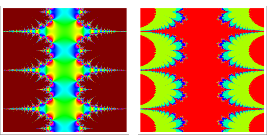
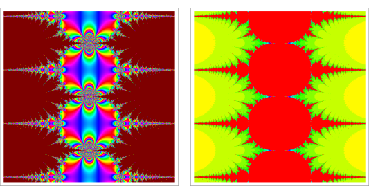
Fixed points of functions in the complex plane commonly lead to beautiful fractal structures. For example, the plots above color the value of the fixed point (left figures) and the number of iterations to reach a fixed point (right figures) for cosine (top) and sine (bottom). Newton's method, which essentially involves a fixed point computation in order to find roots, leads to similar fractals in an analogous way.
Points of an autonomous system of ordinary differential equations at which
 |
(2)
|
are known as fixed points.
If a variable is slightly displaced from a fixed point, it may (1) move back to the fixed point ("asymptotically stable"), (2) move away ("unstable"), or (3) move in a neighborhood of the fixed point but not approach it ("stable" but not "asymptotically stable"). Fixed points are also called critical points or equilibrium points. For an autonomous system with a locally Lipschitz vector field, a trajectory starting away from a fixed point cannot reach it in finite time. Under the same uniqueness hypothesis, a trajectory cannot cross itself unless it is a closed curve, in which case it is a periodic solution.
A fixed point can be classified into one of several classes using linear stability analysis and the resulting stability matrix.
The following table summarizes fixed points of a two-dimensional linear system (Tabor 1989, pp. 22-24). Here  and
 are the eigenvalues
of the stability matrix, and
 ,
 ,
and
 are positive. For a nonlinear system,
purely imaginary eigenvalues of the linearization
alone do not determine stability.
 | fixed point |
 | stable node |
 | unstable node |
 | hyperbolic fixed point |
 | stable spiral point |
 | unstable spiral point |
 | elliptic fixed point |
 ,
two independent eigenvectors | stable star |
 , two independent
eigenvectors | unstable star |
 , one independent eigenvector | stable improper node |
 ,
one independent eigenvector | unstable improper node |
