Heilbronn Triangle Problem

The Heilbronn triangle problem seeks to find a configuration of points in a region of unit area, such as a disk, square, or equilateral triangle, that maximizes the area of the smallest triangle determined by any three of the points. The 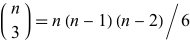points determine triangles. For , there is only a single triangle, so Heilbronn's problem degenerates into finding the largest triangle that can be constructed from points in a square. For , each configuration determines four triangles, and the objective is to maximize their minimum area.

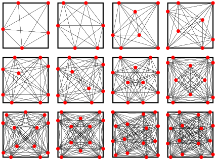
For a unit square, the first few maxima of minimal triangle areas are

			(1)
			(2)
			(3)
			(4)
			(5)
			(6)
			(7)
			(8)

For the unit square, optimality has been proved through : by Yang et al. (1992), by Dress et al. (1995), by Zeng and Chen (2011), by Dehbi and Zeng (2022), and by Sudermann-Merx (2026a), who also gave exact coordinates for all optimal configurations for , ..., 9. For larger values of , proofs of optimality remain open, but the best known results are

			(9)
			(10)
			(11)
			(12)
			(13)
			(14)
			(15)
			(16)
			(17)
			(18)
			(19)
			(20)
			(21)
			(22)
			(23)
			(24)
			(25)
			(26)

with the configurations leading to these minimal triangle areas illustrated above. The configurations associated with these bounds are collected by Friedman and Stead. Earlier sources include Comellas and Yebra (2002) and D. Cantrell and M. Beyleveld (pers. comm., Aug. 16, 2006). Here, the notation indicates a polynomial root. As can be seen, the solutions have a great deal of symmetry, with a large number of maximum minimal triangles sharing the same area.

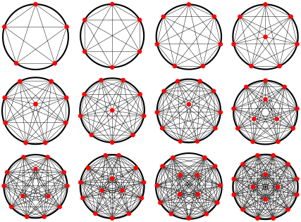
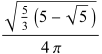
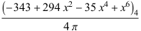
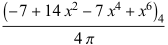
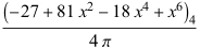
For disks with unit area, the Heilbronn configurations up to 7 are symmetric arrangements of points around the circumference. The best known Heilbronn constants for the circle are

			(27)
			(28)
			(29)
			(30)
			(31)
			(32)
			(33)
			(34)
			(35)
			(36)
			(37)
			(38)
			(39)
			(40)
			(41)
			(42)
			(43)
			(44)
			(45)
			(46)
			(47)
			(48)

(Friedman 2007; D. Cantrell pers. comm., Jun. 18, 2007).

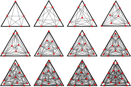
Using an equilateral triangle of unit area instead gives the constants

			(49)
			(50)
			(51)
			(52)
			(53)
			(54)
			(55)
			(56)
			(57)
			(58)
			(59)
			(60)
			(61)
			(62)
			(63)
			(64)
			(65)
			(66)
			(67)
			(68)

Sudermann-Merx (2026b) certified global optimality through and obtained exact optima through . For , the certified numerical optimum agrees to 250 digits with a conjectured root of a degree-7 polynomial. The identification with this root remains conjectural, although the polynomial has galois group . The lower bound is due to AlphaEvolve (Georgiev et al. 2025), and later numerical records are collected by Stead. Earlier values were collected by Friedman and D. Cantrell (pers. comm., Jun. 18, 2007). Friedman also gives a table for the corresponding problem for convex regions of unit area.

Heilbronn conjectured

(69)

but Komlós et al. (1981, 1982) disproved this by showing that

(70)

(Guy 1994, p. 243). For upper bounds, Roth (1951) showed that

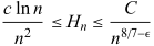(71)

which Schmidt (1971/1972) improved to

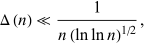(72)

and Roth further improved to

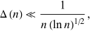(73)

originally with (Roth 1972ab) and later with (Roth 1976; Guy 1994, p. 243). Komlós et al. (1981) obtained , up to a subpolynomial factor, and Cohen et al. (2023) improved the exponent to . Cohen et al. (2024) subsequently proved that, for every ,

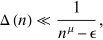(74)

David Cantrell found a heuristic upper bound given by

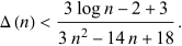(75)