

Christoffel symbols of the second kind are the coefficients of the Levi-Civita connection of a Riemannian metric  in a chosen basis. They are variously denoted as
  (Walton 1967) or
  (Misner et al. 1973, Arfken 1985). They
are also called connection coefficients (Misner et al. 1973, p. 210)
or affine connection coefficients (Weinberg 1972, p. 71).
(Misner et al. 1973, Arfken 1985). They
are also called connection coefficients (Misner et al. 1973, p. 210)
or affine connection coefficients (Weinberg 1972, p. 71).
The coordinate-basis and noncoordinate-basis formulas below give coefficients of the same Levi-Civita connection in different bases. In a coordinate basis, the coefficients can be expressed in terms of the metric tensor alone.
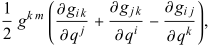
For a coordinate basis, Arfken (1985, p. 161) gives
 |  |  |
(1)
|
 |  | ![g^(km)[ij,k]](/images/equations/ChristoffelSymboloftheSecondKind/Inline9.svg) |
(2)
|
 |  |  |
(3)
|
where  is a partial
derivative,
is a partial
derivative,  is the metric tensor,
and
is the metric tensor,
and  is the corresponding inverse metric,
 |
(4)
|
where  is the radius vector, and
 |
(5)
|
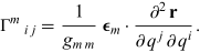
Therefore, for an orthogonal curvilinear coordinate system, by this definition,
 |
(6)
|
Because the coordinate basis vectors commute and the Levi-Civita connection is torsion-free,
 |
(7)
|
(Walton 1967).
This Christoffel symbol of the second kind is related to the Christoffel symbol of the first kind ![[bc,d]](/images/equations/ChristoffelSymboloftheSecondKind/Inline17.svg) by
by
![Gamma^a_(bc)=g^(ad)[bc,d].](/images/equations/ChristoffelSymboloftheSecondKind/NumberedEquation5.svg) |
(8)
|
Walton (1967) lists Christoffel symbols of the second kind for the 12 basic orthogonal coordinate systems.
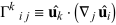
For an orthonormal basis  that need not be a coordinate basis, Misner et al.
(1973, p. 209) give the coefficients as
that need not be a coordinate basis, Misner et al.
(1973, p. 209) give the coefficients as
 |
(9)
|
where  denotes the covariant
derivative in the direction of
denotes the covariant
derivative in the direction of  . These coefficients need not be symmetric in
  and
and  because the basis vectors
need not commute.
because the basis vectors
need not commute.
Christoffel symbols of the second kind are not tensors and do not transform as tensor components. For two coordinate bases related by a
change from  to
to  , the transformation law is
 |
(10)
|
Here the lowered-index convention is  . For
the Levi-Civita connection in a general
basis, these coefficients are
. For
the Levi-Civita connection in a general
basis, these coefficients are
 |
(11)
|
(Misner et al. 1973, p. 210), where the  s are components of the metric
tensor,
s are components of the metric
tensor,  for the commutation
coefficients
for the commutation
coefficients ![[e_alpha,e_beta]=c_(alphabeta)^mue_mu](/images/equations/ChristoffelSymboloftheSecondKind/Inline28.svg) , and the commas indicate
the comma derivative. In a coordinate basis,
the commutation coefficients vanish and
this reduces to a Christoffel symbol
of the first kind. In an orthonormal basis,
the metric components are constant, so
, and the commas indicate
the comma derivative. In a coordinate basis,
the commutation coefficients vanish and
this reduces to a Christoffel symbol
of the first kind. In an orthonormal basis,
the metric components are constant, so  and
and  . Hence
 |
(12)
|
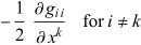
For an orthogonal coordinate basis, in contrast, the metric is diagonal but its diagonal components need not be constant. In this setting,
 |  |  |
(13)
|
 |  |  |
(14)
|
 |  |  |
(15)
|
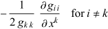 |  |  |
(16)
|
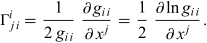 |  |  |
(17)
|
 |  |  |
(18)
|
In three dimensions, the Christoffel symbols of the second kind may be arranged in matrix form:
![Gamma^l=[Gamma^l_(ii) Gamma^l_(ij) Gamma^l_(ik); Gamma^l_(ji) Gamma^l_(jj) Gamma^l_(jk); Gamma^l_(ki) Gamma^l_(kj) Gamma^l_(kk)].](/images/equations/ChristoffelSymboloftheSecondKind/NumberedEquation10.svg) |
(19)
|
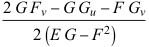
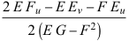
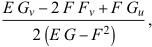
The Christoffel symbols are given in terms of the coefficients of the first fundamental form 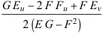 ,
,  , and
, and  by
by
 |  |  |
(20)
|
 |  |  |
(21)
|
 |  |  |
(22)
|
 |  |  |
(23)
|
 |  |  |
(24)
|
 |  |  |
(25)
|
and  and
and  .
If
.
If  ,
the Christoffel symbols of the second kind simplify to
,
the Christoffel symbols of the second kind simplify to
 |  |  |
(26)
|
 |  |  |
(27)
|
 |  |  |
(28)
|
 |  |  |
(29)
|
 |  |  |
(30)
|
 |  |  |
(31)
|
(Gray 1997).
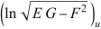
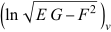
The following relationships hold between the Christoffel symbols of the second kind and coefficients of the first fundamental form,
 |  |  |
(32)
|
 |  |  |
(33)
|
 |  |  |
(34)
|
 |  |  |
(35)
|
 |  |  |
(36)
|
 |  |  |
(37)
|
 |  | 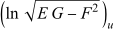 |
(38)
|
 |  | 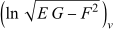 |
(39)
|
(Gray 1997).
For a surface given in Monge's form  ,
,
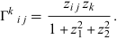 |
(40)
|
Christoffel symbols of the second kind arise in the computation of geodesics. The geodesic equation of free motion is
 |
(41)
|
or
 |
(42)
|
Expanding,
 |
(43)
|
 |
(44)
|
But
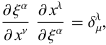 |
(45)
|
so
 |
(46)
|
where
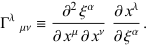 |
(47)
|
