

A contingency table, sometimes called a two-way frequency table, is a tabular mechanism with at least two rows and two columns used in statistics
to present categorical data in terms of frequency
counts. More precisely, an  contingency table shows the observed frequency of two
variables, the observed frequencies of which are arranged
into
contingency table shows the observed frequency of two
variables, the observed frequencies of which are arranged
into  rows and
  columns. The intersection of a row and a column of a contingency table is called
a cell.
columns. The intersection of a row and a column of a contingency table is called
a cell.
| gender | cup | cone | sundae | sandwich | other |
| male | 592 | 300 | 204 | 24 | 80 |
| female | 410 | 335 | 180 | 20 | 55 |
For example, the above contingency table has two rows and five columns (not counting header rows/columns) and shows the results of a random sample of  adults classified by two variables, namely gender and favorite
way to eat ice cream (Larson and Farber 2014). One benefit of having data presented
in a contingency table is that it allows one to more easily perform basic probability
calculations, a feat made easier still by augmenting a summary row and column to
the table.
adults classified by two variables, namely gender and favorite
way to eat ice cream (Larson and Farber 2014). One benefit of having data presented
in a contingency table is that it allows one to more easily perform basic probability
calculations, a feat made easier still by augmenting a summary row and column to
the table.
| gender | cup | cone | sundae | sandwich | other | total |
| male | 592 | 300 | 204 | 24 | 80 | 1200 |
| female | 410 | 335 | 180 | 20 | 55 | 1000 |
| total | 1002 | 635 | 384 | 44 | 135 | 2200 |
The above table is an extended version of the first table obtained by adding a summary row and column. These summaries allow easier computation of several different probability-related quantities. For example, the estimated
probability that a person in the sampled population prefers ice cream in a cup is
 , while the estimated
probability that a random participant is female is
, while the estimated
probability that a random participant is female is  . Computing conditional
probabilities is also made easier using contingency tables. For example, the
probability that a person prefers ice cream sandwiches given that the person is male
is
. Computing conditional
probabilities is also made easier using contingency tables. For example, the
probability that a person prefers ice cream sandwiches given that the person is male
is  ,
while the conditional probability that a person is male given that ice cream sandwiches
are preferred is
,
while the conditional probability that a person is male given that ice cream sandwiches
are preferred is  .
.
Other common statistical analyses can be performed on data given in contingency table form. Let  be the total of row
  ,
,
 the total of column
  ,
and
,
and  the sample size. The expected frequency
  of the cell at their intersection under independence
is
of the cell at their intersection under independence
is
 |
(1)
|
Computing  says that the value one would expect at cell
  --i.e., the expected number of men who prefer to eat ice
cream from a cup--is approximately
--i.e., the expected number of men who prefer to eat ice
cream from a cup--is approximately
 |
(2)
|
so the observed count 592 is greater than the expected count under independence. Knowing  also gives
  without repeated application of (1):
 |
(3)
|
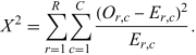
One of the major benefits of computing expected frequencies is the ability to test whether the two variables being examined--in this case, gender and favorite way to
eat ice cream--are independent. This is done by computing, for each cell  , the expected frequency
  , comparing it to the observed frequency
  , and then performing a chi-squared
test. For an
, and then performing a chi-squared
test. For an  table, the Pearson statistic is
 |
(4)
|
Under the null hypothesis of independence and the usual large-sample conditions,  has approximately a chi-squared
distribution with
has approximately a chi-squared
distribution with  degrees of freedom.
Its upper-tail probability is the P-value for
the chi-squared test. Individual cell frequencies
can also be divided by the sample size to estimate cell probabilities, with uncertainty
summarized by an appropriate confidence interval
under a binomial distribution or multinomial
distribution model.
degrees of freedom.
Its upper-tail probability is the P-value for
the chi-squared test. Individual cell frequencies
can also be divided by the sample size to estimate cell probabilities, with uncertainty
summarized by an appropriate confidence interval
under a binomial distribution or multinomial
distribution model.
Another common test associated with contingency tables is the homogeneity of proportions test, a form of chi-squared test used to determine whether several proportions are equal when samples are taken from different populations (Larson and Farber 2014). The usual large-sample rule of thumb for these chi-squared approximations calls for randomly selected observations and expected frequencies of at least 5 in each cell. These tests play important roles throughout various branches of statistics.
