

Vector spherical harmonics generalize spherical harmonics to vector-valued functions. They can be constructed by looking for
a scalar function  and a constant vector
  such that
 |  |  |
(1)
|
 |  |  |
(2)
|
 |  |  |
(3)
|
 |  |  |
(4)
|
so
 |
(5)
|
Now interchange the order of differentiation and use the fact that multiplicative constants can be moving inside and outside the derivatives to obtain
 |  |  |
(6)
|
 |  |  |
(7)
|
 |  |  |
(8)
|
and
 |  |  |
(9)
|
 |  |  |
(10)
|
Putting these together gives
![del ^2M+k^2M=del x[c(del ^2psi+k^2psi)],](/images/equations/VectorSphericalHarmonic/NumberedEquation2.svg) |
(11)
|
so  satisfies the vector Helmholtz differential
equation if
satisfies the vector Helmholtz differential
equation if  satisfies the scalar Helmholtz
differential equation
satisfies the scalar Helmholtz
differential equation
 |
(12)
|
Construct another vector function
 |
(13)
|
which also satisfies the vector Helmholtz differential equation since
 |  |  |
(14)
|
 |  |  |
(15)
|
 |  |  |
(16)
|
 |  |  |
(17)
|
 |  |  |
(18)
|
which gives
 |
(19)
|
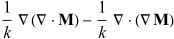
We have the additional identity
 |  |  |
(20)
|
 |  |  |
(21)
|
 |  |  |
(22)
|
 |  |  |
(23)
|
 |  |  |
(24)
|
In this formalism,  is called the generating function and
  is called the pilot vector. The choice of generating function
is determined by the symmetry of the scalar equation, i.e., it is chosen to solve
the desired scalar differential equation. If
is called the pilot vector. The choice of generating function
is determined by the symmetry of the scalar equation, i.e., it is chosen to solve
the desired scalar differential equation. If  is taken as
 |
(25)
|
where  is the radius vector, then
  is a solution to the vector wave equation in spherical coordinates.
If we want vector solutions which are tangential to the radius vector,
is a solution to the vector wave equation in spherical coordinates.
If we want vector solutions which are tangential to the radius vector,
 |  |  |
(26)
|
 |  |  |
(27)
|
 |  |  |
(28)
|
so
 |
(29)
|
and we may take
 |
(30)
|
(Arfken 1985, pp. 707-711; Bohren and Huffman 1983, p. 88).
A number of conventions are in use. Hill (1954) defines
 |  |  |
(31)
|
 |  |  |
(32)
|
 |  |  |
(33)
|
Morse and Feshbach (1953) define vector harmonics called  ,
,  , and
, and  using rather complicated expressions.
