Euler Differential Equation -- from Wolfram MathWorld

The nonhomogeneous Euler differential equation is

(1)

and the homogeneous equation is

(2)

(3)

Now attempt to convert the equation from

(4)

to one with constant coefficients

(5)

by using the standard transformation for linear second-order ordinary differential equations. Comparing (3) and (5), the functions and are

(6)

(7)

Let and define

			(8)
			(9)
			(10)
			(11)

Then is given by

			(12)
			(13)
			(14)

which is a constant. Therefore, the equation becomes a second-order ordinary differential equation with constant coefficients

(15)

Define

			(16)
			(17)
			(18)
			(19)

and

			(20)
			(21)

The solutions are

$y={c_1e^(r_1z)+c_2e^(r_2z) (alpha-1)^2>4beta; (c_1+c_2z)e^(az) (alpha-1)^2=4beta; e^(az)[c_1cos(bz)+c_2sin(bz)] (alpha-1)^2<4beta.$

(22)

In terms of the original variable ,

$y={c_1|x|^(r_1)+c_2|x|^(r_2) (alpha-1)^2>4beta; (c_1+c_2ln|x|)|x|^a (alpha-1)^2=4beta; |x|^a[c_1cos(bln|x|)+c_2sin(bln|x|)] (alpha-1)^2<4beta.$

(23)

For and a continuous function on , the nonhomogeneous equation has general solution , where is the corresponding homogeneous solution above. When , a particular solution is

(24)

For the repeated root , it is

(25)

Zwillinger (1997, p. 120) gives two other types of equations known as Euler differential equations,

(26)

(Valiron 1950, p. 201) and

(27)

(Valiron 1950, p. 212), the latter of which can be solved in terms of Bessel functions. The substitution reduces the latter Riccati differential equation to . For and , putting gives

(28)

where is a Bessel function of the first kind and is a Bessel function of the second kind. This representation holds locally away from , using consistent branches, and requires . For , take 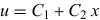. For , the equation for is an Euler differential equation of the homogeneous form above.

Euler Differential Equation

See also

Explore with Wolfram|Alpha

References

Referenced on Wolfram|Alpha

Cite this as:

Subject classifications