Conformal Mapping

A conformal mapping, also called a conformal map, conformal transformation, or angle-preserving transformation, is a transformation that preserves local oriented angles. An analytic function is conformal at any point where it has a nonzero derivative. Conversely, any conformal mapping of a complex variable which has continuous partial derivatives is analytic. Conformal mapping is extremely important in complex analysis, as well as in many areas of physics and engineering.

A mapping that preserves the magnitude of angles, but not their orientation is called an isogonal mapping (Churchill and Brown 1990, p. 241).

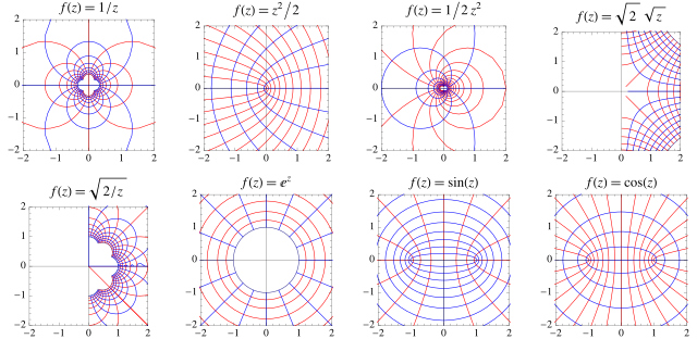
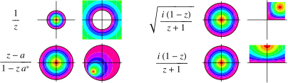
Several conformal transformations of regular grids are illustrated in the first figure above. In the second figure above, contours of constant are shown together with their corresponding contours after the transformation. Moon and Spencer (1988) and Krantz (1999, pp. 183-194) give tables of conformal mappings.

A method due to Szegö gives an iterative approximation to the conformal mapping of a square to a disk, and an exact mapping can be done using elliptic functions (Oberhettinger and Magnus 1949; Trott 2004, pp. 71-77).

Let and be the tangents to the curves and at and in the complex plane,

			(1)
			(2)

(3)

Then as and ,

(4)

(5)

A function is a conformal bijection iff there are complex numbers and such that

(6)

for (Krantz 1999, p. 80). Furthermore, if is an analytic function such that

(7)

then is a polynomial in (Greene and Krantz 1997; Krantz 1999, p. 80).

Conformal transformations can prove extremely useful in solving physical problems. By letting , the real part and imaginary part of must satisfy the Cauchy-Riemann equations and Laplace's equation, so they automatically provide a scalar potential and a so-called stream function. If a physical problem can be found for which the solution is valid, we obtain a solution--which may have been very difficult to obtain directly--by working backwards.

For example, let

(8)

where is a real constant, is real, and . The real part and imaginary part then give

			(9)
			(10)

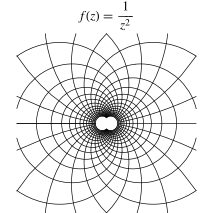
For ,

			(11)
			(12)

which is a double system of lemniscates (Lamb 1945, p. 69).

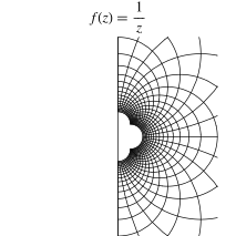
For ,

			(13)
			(14)

This solution consists of two systems of circles, and is the potential function for two parallel opposite charged line charges (Lamb 1945, p. 69; Feynman et al. 1989, §7-5).

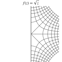
For and ,

			(15)
			(16)

gives the field near the edge of a thin plate (Feynman et al. 1989, §7-5).

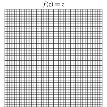
For ,

			(17)
			(18)

giving two straight lines (Lamb 1945, p. 68).

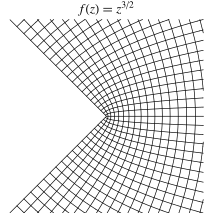
For ,

(19)

gives the field near the outside of a rectangular corner (Feynman et al. 1989, §7-5).

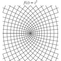
For ,

			(20)
			(21)
			(22)

These are two perpendicular hyperbolas, and is the potential function near the middle of two point charges or the field on the opening side of a charged right angle conductor (Feynman 1989, §7-3).