TOPICS
Search

Lebesgue Constants


The term "Lebesgue constants" refers to either of two commonly used sets. The first is related to approximation of functions via Fourier series, while the other arises in the computation of Lagrange interpolating polynomials.

Assume a function f(x) is integrable over the interval [-pi,pi] and S_n(f,x) is the nth partial sum of the Fourier series of f, so that

a_k=1/piint_(-pi)^pif(t)cos(kt)dt
(1)
b_k=1/piint_(-pi)^pif(t)sin(kt)dt
(2)

and

 S_n(f,x)=1/2a_0+{sum_(k=1)^n[a_kcos(kx)+b_ksin(kx)]}.
(3)

If

 |f(x)|<=1
(4)

for all x, then

 |S_n(f,x)|<=1/piint_0^pi(|sin[1/2(2n+1)theta]|)/(sin(1/2theta))dtheta=L_n,
(5)

and L_n is the smallest possible constant for which this holds for all continuous functions f(x). The first few values of L_n are

L_0=1
(6)
L_1=1/3+(2sqrt(3))/pi
(7)
=1.435991124...
(8)
L_2=1/5+(sqrt(25-2sqrt(5)))/pi=1.642188435...
(9)
L_3=1/7+1/(3pi)[22sin(pi/7)-2cos(pi/(14))+10cos((3pi)/(14))]
(10)
=1.778322861...
L_4=(13)/(2sqrt(3)pi)+1/9+1/pi[7sin((2pi)/9)-5sin(pi/9)-cos(pi/(18))]
(11)
=1.880080599....
(12)

Some sum formulas for L_n include

L_n=1/(2n+1)+2/pisum_(k=1)^(n)1/ktan((pik)/(2n+1))
(13)
=(16)/(pi^2)sum_(k=1)^(infty)sum_(j=1)^((2n+1)k)1/(4k^2-1)1/(2j-1)
(14)

(Zygmund 1959) and integral formulas include

L_n=4int_0^infty(tanh[(2n+1)x])/(tanhx)(dx)/(pi^2+4x^2)
(15)
=4/(pi^2)int_0^infty(sinh[(2n+1)x])/(sinhx)ln{coth[1/2(2n+1)x]}dx
(16)

(Hardy 1942). For large n,

 4/(pi^2)lnn<L_n<3+4/(pi^2)lnn.
(17)

This result can be generalized for a 2pi-periodic function with r continuous derivatives, where r>=1 is an integer, satisfying

 |(d^rf)/(dx^r)|<=1
(18)

for all x. In this case,

 |f(x)-S_n(f,x)|<=L_(n,r)=4/(pi^2)(lnn)/(n^r)+O(1/(n^r)),
(19)

where

 L_(n,r)={1/piint_(-pi)^pi|sum_(k=n+1)^(infty)(sin(kx))/(k^r)|dx   for r>=1 odd; 1/piint_(-pi)^pi|sum_(k=n+1)^(infty)(cos(kx))/(k^r)|dx   for r>=1 even
(20)

(Kolmogorov 1935, Zygmund 1959).

Watson (1930) showed that

 lim_(n->infty)[L_n-4/(pi^2)ln(2n+1)]=c,
(21)

where

c=8/(pi^2)(sum_(k=1)^(infty)(lnk)/(4k^2-1))-4/(pi^2)(Gamma^'(1/2))/(Gamma(1/2))
(22)
=8/(pi^2)[sum_(j=0)^(infty)(lambda(2j+2)-1)/(2j+1)]+4/(pi^2)(2ln2+gamma)
(23)
=0.9894312738...
(24)

(OEIS A243277), where Gamma(z) is the gamma function, lambda(z) is the Dirichlet lambda function, and gamma is the Euler-Mascheroni constant.

For a positive integer n and n distinct nodes X={x_1,...,x_n} with -1<=x_1<...<x_n<=1, define the nth Lebesgue constant for the Lagrange interpolating polynomial by

 Lambda_n(X)=max_(-1<=x<=1)sum_(k=1)^n|product_(j!=k)(x-x_j)/(x_k-x_j)|.
(25)

It is then true that

 Lambda_n>4/(pi^2)lnn-1.
(26)

The efficiency of Lagrange interpolating polynomial approximation is related to the rate at which Lambda_n increases. Erdős (1961) proved that there exists a positive constant such that

 Lambda_n>2/pilnn-C
(27)

for all n. For the nodes given by the roots of the Chebyshev polynomial of the first kind T_n, Erdős (1961) notes that

 Lambda_n(X)<2/pilnn+C_2,
(28)

where C_2 is a positive constant independent of n. Thus the leading coefficient of lnn in (27) cannot be increased.

A node set X is called canonical when it contains both endpoints -1 and 1. For n>=3, there is a unique canonical set minimizing Lambda_n(X). It is symmetric about 0, and its Lebesgue function attains the same maximum on each of the n-1 intervals between successive nodes. These Bernstein-Erdős theorems were established by Kilgore (1977, 1978) and de Boor and Pinkus (1978). More precisely, let m(X) and M(X) be the smallest and largest of those interval maxima, and let Lambda_n^* be the optimal value. Then

 m(X)<=Lambda_n^*<=M(X),
(29)

with both inequalities strict for every other canonical set.

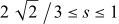
The endpoint condition is essential to the uniqueness assertion. Without it, every three-node set X={-s,0,s} with 2sqrt(2)/3<=s<=1 has the minimal value Lambda_3(X)=5/4. Indeed, writing u=|x|/s, its Lebesgue function is 1+u-u^2 for 0<=u<=1 and 2u^2-1 for u>=1, so

 Lambda_3({-s,0,s})=max(5/4,2/(s^2)-1).
(30)

See also

Chebyshev Polynomial of the First Kind, Fourier Series, Lagrange Interpolating Polynomial

Explore with Wolfram|Alpha

References

de Boor, C. and Pinkus, A. "Proof of the Conjectures of Bernstein and Erdős Concerning the Optimal Nodes for Polynomial Interpolation." J. Approx. Th. 24, 289-303, 1978. https://doi.org/10.1016/0021-9045(78)90014-X.Erdős, P. "Problems and Results on the Theory of Interpolation, II." Acta Math. Acad. Sci. Hungary 12, 235-244, 1961.Finch, S. R. "Lebesgue Constants." §4.2 in Mathematical Constants. Cambridge, England: Cambridge University Press, pp. 250-255, 2003.Hardy, G. H. "Note on Lebesgue's Constants in the Theory of Fourier Series." J. London Math. Soc. 17, 4-13, 1942.Kilgore, T. A. "Optimization of the Norm of the Lagrange Interpolation Operator." Bull. Amer. Math. Soc. 83, 1069-1071, 1977.Kilgore, T. A. "A Characterization of the Lagrange Interpolating Projection with Minimal Tchebycheff Norm." J. Approx. Th. 24, 273-288, 1978. https://doi.org/10.1016/0021-9045(78)90013-8.Kolmogorov, A. N. "Zur Grössenordnung des Restgliedes Fourierscher reihen differenzierbarer Funktionen." Ann. Math. 36, 521-526, 1935.Sloane, N. J. A. Sequence A243277 in "The On-Line Encyclopedia of Integer Sequences."Watson, G. N. "The Constants of Landau and Lebesgue." Quart. J. Math. Oxford 1, 310-318, 1930.Zygmund, A. G. Trigonometric Series, 2nd ed., Vols. 1-2. Cambridge, England: Cambridge University Press, 1959.

Referenced on Wolfram|Alpha

Lebesgue Constants

Cite this as:

Weisstein, Eric W. "Lebesgue Constants." From MathWorld--A Wolfram Resource. https://mathworld.wolfram.com/LebesgueConstants.html

Subject classifications