Laplace Limit

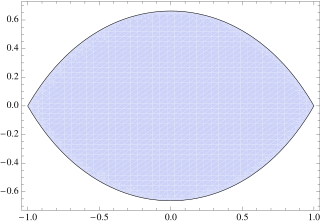
The Laplace limit is the greatest orbital eccentricity for which Laplace's series solution of Kepler's equation converges for every real mean anomaly.

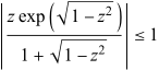
For a complex number with , the inequality

describes the lens-shaped region illustrated above, using the principal square root. The restriction excludes the real rays beyond , where the displayed complex modulus also equals 1. In terms of real variables, the same region is described by

where

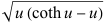
The first-quadrant boundary of this region can be parameterized for as

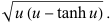
Written parametrically in terms of the Cartesian coordinates,

The values at are defined by continuity. Reflections in the coordinate axes give the remaining boundary. The parameter has maximum value (OEIS A085984; Le Lionnais 1983, p. 36), the unique positive root of

or equivalently of

Goursat (1959, p. 120) credits Stieltjes with the numerical value.

By symmetry, the area enclosed is therefore

Another exact reduction is obtained by defining and pairing two values and on the physical reflection sheet so that . With , this equation factors as

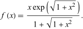
where is defined to be 1 at . The first component is , or . Although explicit, it is not the physical reflection sheet. At the cubic cusp , continuation of the physical area switches instead to the nontrivial component

On the nontrivial component, define and

For , , while at . Together, these relations give , the ordinary transition between the and branches of the Lambert W-function studied by Åhag et al. (2024).

Setting

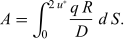
with for gives the exact area representation

Equivalently, this is the explicit integral

which agrees numerically with the parametrized formula above. Here is an associated Laguerre polynomial, also called a generalized Laguerre polynomial. An exact series representation for the area is

(OEIS A140133; E. Weisstein, Aug. 27, 2026). While the preceding representations are exact, they do not constitute a finite closed form free of both integration and an infinite sum.

This region is intimately related to the study of Bessel functions and Kapteyn series (Plummer 1960, p. 47; Watson 1966, p. 270).

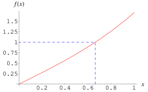
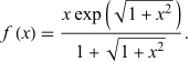
The minimum value of corresponding to the maximum value is (OEIS A033259; Plummer 1960, p. 47; Watson 1966, p. 270), which is known as the Laplace limit constant. It is the convergence threshold for Laplace's series solution of Kepler's equation and is the unique real number satisfying , where

The same constant controls the existence of a catenoid spanning two equal coaxial circles of radius whose planes are separated by a distance : such a catenoid exists only for . At equality it is the critical catenoid, and the volume bounded by the catenoid and its two boundary disks is (Anderson 2026).

The continued fraction of is given by [0, 1, 1, 1, 27, 1, 1, 1, 8, 2, 154, ...] (OEIS A033260). Counting the initial zero at position 1, the positions of the first occurrences of in the continued fraction of are 2, 10, 35, 13, 15, 32, 101, 9, ... (OEIS A033261). The incrementally largest terms in the continued fraction are 1, 27, 154, 1601, 2135, ... (OEIS A033262), which occur at positions 2, 5, 11, 19, 1801, ... (OEIS A033263). The displayed positions are one greater than the zero-based positions in OEIS A033261 and OEIS A033263.