


The name Heawood four-color map is used here for Heawood's (1890) map and its later variants, and for their associated graphs.
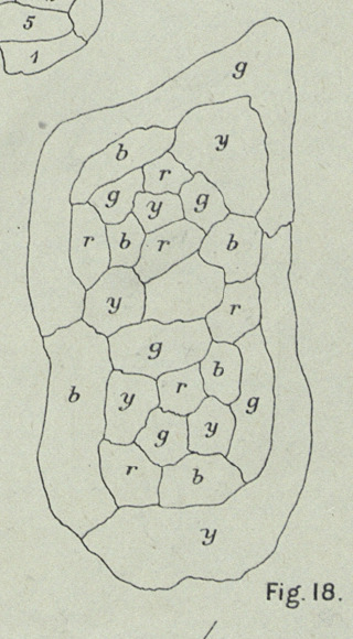
Heawood's (1890, pp. 337-338, Plate 3, Fig. 18) map, illustrated above, provides a counterexample to Kempe's (1879) supposed proof of the four-color theorem.
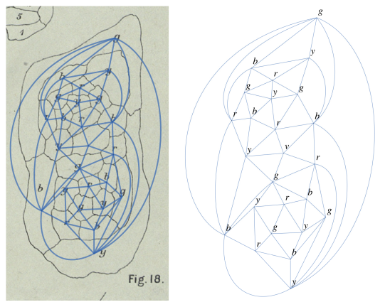
The graph formed by representing each region of the map by a vertex and joining vertices
whose regions share a boundary line segment is a planar
graph with 25 vertices and 69 edges.
Its vertex degrees are 5, 6, and 7 with multiplicities
16, 5, and 4, respectively. The originally blank country is labeled  in the corresponding graph drawing
above. Heawood's original version will be implemented in the a future version of
the Wolfram Language as GraphData["HeawoodFourColorMapGraph"].
in the corresponding graph drawing
above. Heawood's original version will be implemented in the a future version of
the Wolfram Language as GraphData["HeawoodFourColorMapGraph"].
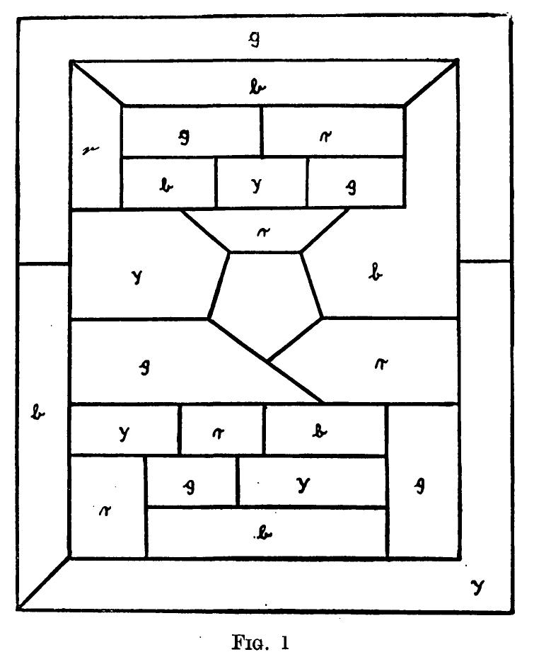
Dirac (1963, p. 269, Fig. 1) gives a rectangular version of Heawood's map in which the boundary between the outer green and outer blue countries differs from that in Heawood's original map (1890). In particular, the outer green country shares a boundary line segment with the middle yellow country, while the upper red country no longer shares a boundary line segment with the outer blue country. This gives one edge added and another removed relative to the graph formed from Heawood's original map. The figure also omits the boundary separating the upper-right yellow country from the blue country beside the central blank country in Heawood's original map, joining them into a single blue country. Dirac gives no indication that his boundaries differ from Heawood's, nor does he explain why they do so. He discusses the figure by quoting Heawood's explanation of why Kempe's argument fails (Dirac 1963, p. 270).
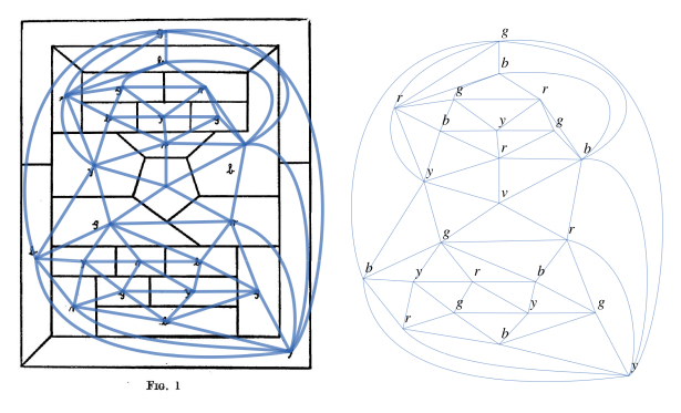
The graph corresponding to Dirac's map, illustrated above, has 24 vertices and 66 edges, whose vertex degrees are 4, 5, 6, 7, and 8 with multiplicities 1, 15, 4, 3, and 1, respectively. Dirac's version will be implemented in the a future version of the Wolfram Language as GraphData["DiracFourColorMapGraph"].
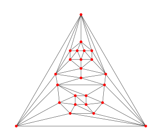
Saaty's (1972, p. 9, Fig. 4) version, illustrated above, also has 25 vertices and 69 edges, but its vertex degrees are 5, 6, and 7 with multiplicities 17, 3, and 5, respectively. The same graph is illustrated as "Heawood" by Gethner et al. (2009, p. 255, Fig. 2). Saaty's version of the Heawood four-color map is implemented in the Wolfram Language as GraphData["HeawoodFourColorGraph"] and will be implemented in the a future version of the Wolfram Language as GraphData["SaatyFourColorMapGraph"]. Restoring the omitted boundary in Dirac's map separates its large upper-right blue country into the yellow and blue countries of Heawood's original map. The resulting graph has 25 vertices and 69 edges and is isomorphic to Saaty's graph. Saaty's reference to Heawood (1890) also cites Dirac (1963).
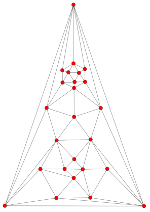
Another graph, labeled "Heawood's counter example in graph form," is given by Soifer (2024, pp. 221-222, Fig. 21.4) and illustrated above. It has 25 vertices and 67 edges. Its vertex degrees are 4, 5, 6, and 7 with multiplicities 4, 12, 5, and 4, respectively. Soifer credits Saaty (1972, p. 9) with translating Heawood's map into graph form and adding symmetry. He presents the drawing as a drawing of Saaty's graph, developed with Phillip Emerich using regular hexagons and pentagons. However, the illustrated 67-edge graph is distinct from Saaty's 69-edge version (as well as distinct from the nine-vertex Soifer graph). Soifer's version will be implemented in the a future version of the Wolfram Language as GraphData["SoiferFourColorMapGraph"].
The following table compares these four versions. Here  and
and  are the numbers of vertices
and edges, respectively. Each version is a planar
graph and a counterexample to Kempe's
coloring algorithm.
are the numbers of vertices
and edges, respectively. Each version is a planar
graph and a counterexample to Kempe's
coloring algorithm.
| version |  |  | planar | Kempe counterexample | vertex degree polynomial |
| Dirac (1963) | 24 | 66 | true | true |  |
| Heawood (1890) | 25 | 69 | true | true |  |
| Saaty (1972) | 25 | 69 | true | true |  |
| Soifer (2024) | 25 | 67 | true | true |  |
The Fritsch graph and Soifer graph provide smaller (and in fact the smallest possible) counterexamples.
