The spherical harmonics Laplace's equation in spherical
coordinates where azimuthal symmetry is not present. Some care must be taken
in identifying the notational convention being used. In this entry, Wolfram
Language (in mathematical literature, Wolfram Language as SphericalHarmonicY l ,
m , theta , phi ].
Spherical harmonics satisfy the spherical harmonic differential equation , which is given by the angular part of Laplace's
equation in spherical coordinates . Writing
(1)
Multiplying by
(2)
Using separation of variables by equating the
(3)
which has solutions
(4)
Plugging in (3 ) into (2 ) gives the equation for the
(5)
where associated Legendre polynomial .
The spherical harmonics are then defined by combining
(6)
where the normalization is chosen such that
(7)
(Arfken 1985, p. 681). Here, complex conjugate
and Kronecker delta . Sometimes (e.g., Arfken
1985), the Condon-Shortley phase
The spherical harmonics are sometimes separated into their real
and imaginary parts ,
(8)
(9)
The spherical harmonics obey
where Legendre polynomial .
Integrals of products of three spherical harmonics, also known as Gaunt
coefficients , are given by
(13)
where Wigner 3j -symbol (which is related
to the Clebsch-Gordan coefficients ).
Special cases include
(Arfken 1985, p. 700).
The above illustrations show
Written in terms of Cartesian coordinates ,
so
The zonal harmonics are defined to be those of the form
(43)
The tesseral harmonics are those of
the form
(44)
(45)
for sectorial harmonics are of
the form
(46)
(47)
See also Associated Legendre Polynomial ,
Condon-Shortley Phase ,
Correlation Coefficient ,
Gaunt
Coefficient ,
Laplace Series ,
Sectorial
Harmonic ,
Solid Harmonic ,
Spherical
Harmonic Addition Theorem ,
Spherical
Harmonic Differential Equation ,
Spherical
Harmonic Closure Relations ,
Surface Harmonic ,
Tesseral Harmonic ,
Vector
Spherical Harmonic ,
Zonal Harmonic
Related Wolfram sites https://functions.wolfram.com/Polynomials/SphericalHarmonicY/ ,
https://functions.wolfram.com/HypergeometricFunctions/SphericalHarmonicYGeneral/
Explore with Wolfram|Alpha
References Abbott, P. "2. Schrödinger Equation." Lecture Notes for Computational Physics 2. http://physics.uwa.edu.au/pub/Computational/CP2/2.Schroedinger.nb . Arfken,
G. "Spherical Harmonics" and "Integrals of the Products of Three Spherical
Harmonics." §12.6 and 12.9 in Mathematical
Methods for Physicists, 3rd ed. Byerly, W. E. "Spherical Harmonics."
Ch. 6 in An
Elementary Treatise on Fourier's Series, and Spherical, Cylindrical, and Ellipsoidal
Harmonics, with Applications to Problems in Mathematical Physics. Ferrers, N. M. An
Elementary Treatise on Spherical Harmonics and Subjects Connected with Them. Groemer, H. Geometric
Applications of Fourier Series and Spherical Harmonics. Hobson, E. W. The
Theory of Spherical and Ellipsoidal Harmonics. Kalf,
H. "On the Expansion of a Function in Terms of Spherical Harmonics in Arbitrary
Dimensions." Bull. Belg. Math. Soc. Simon Stevin 2 , 361-380, 1995. MacRobert,
T. M. and Sneddon, I. N. Spherical
Harmonics: An Elementary Treatise on Harmonic Functions, with Applications, 3rd ed.
rev. Normand, J. M.
A
Lie Group: Rotations in Quantum Mechanics. Press, W. H.; Flannery, B. P.; Teukolsky, S. A.;
and Vetterling, W. T. "Spherical Harmonics." §6.8 in Numerical
Recipes in FORTRAN: The Art of Scientific Computing, 2nd ed. Sansone, G. "Harmonic
Polynomials and Spherical Harmonics," "Integral Properties of Spherical
Harmonics and the Addition Theorem for Legendre Polynomials," and "Completeness
of Spherical Harmonics with Respect to Square Integrable Functions." §3.18-3.20
in Orthogonal
Functions, rev. English ed. Sternberg,
W. and Smith, T. L. The
Theory of Potential and Spherical Harmonics, 2nd ed. Wang, J.; Abbott, P.; and Williams, J. "Visualizing
Atomic Orbitals." http://physics.uwa.edu.au/pub/Orbitals . Weisstein,
E. W. "Books about Spherical Harmonics." http://www.ericweisstein.com/encyclopedias/books/SphericalHarmonics.html . Whittaker,
E. T. and Watson, G. N. "Solution of Laplace's Equation Involving
Legendre Functions" and "The Solution of Laplace's Equation which Satisfies
Assigned Boundary Conditions at the Surface of a Sphere." §18.31 and 18.4
in A
Course in Modern Analysis, 4th ed. Zwillinger, D. Handbook
of Differential Equations, 3rd ed. Referenced on Wolfram|Alpha Spherical Harmonic
Cite this as:
Weisstein, Eric W. "Spherical Harmonic."
From MathWorld https://mathworld.wolfram.com/SphericalHarmonic.html
Subject classifications
 are the angular portion of the solution to
Laplace's equation in spherical
coordinates where azimuthal symmetry is not present. Some care must be taken
in identifying the notational convention being used. In this entry,
are the angular portion of the solution to
Laplace's equation in spherical
coordinates where azimuthal symmetry is not present. Some care must be taken
in identifying the notational convention being used. In this entry,  is taken as the polar (colatitudinal) coordinate with
![theta in [0,pi]](/images/equations/SphericalHarmonic/Inline3.svg) ,
and
,
and  as the azimuthal (longitudinal) coordinate with
  . This is the convention normally used in physics,
as described by Arfken (1985) and the Wolfram
Language (in mathematical literature,
. This is the convention normally used in physics,
as described by Arfken (1985) and the Wolfram
Language (in mathematical literature,  usually denotes the longitudinal coordinate and
  the colatitudinal coordinate). Spherical harmonics are implemented
in the Wolfram Language as SphericalHarmonicY[l,
m, theta, phi].
the colatitudinal coordinate). Spherical harmonics are implemented
in the Wolfram Language as SphericalHarmonicY[l,
m, theta, phi].
 in this equation gives

 gives
gives
![[(sintheta)/(Theta(theta))d/(dtheta)(sintheta(dTheta)/(dtheta))+l(l+1)sin^2theta]+1/(Phi(phi))(d^2Phi(phi))/(dphi^2)=0.](/images/equations/SphericalHarmonic/NumberedEquation2.svg)
 -dependent
portion to a constant gives
-dependent
portion to a constant gives


 -dependent
portion, whose solution is
-dependent
portion, whose solution is

 ,
,
 ,
..., 0, ...,
,
..., 0, ...,  ,
,
 and
and  is an associated Legendre polynomial.
The spherical harmonics are then defined by combining
is an associated Legendre polynomial.
The spherical harmonics are then defined by combining  and
and  ,
,


 denotes the complex conjugate
and
denotes the complex conjugate
and  is the Kronecker delta. Sometimes (e.g., Arfken
1985), the Condon-Shortley phase
is the Kronecker delta. Sometimes (e.g., Arfken
1985), the Condon-Shortley phase  is prepended to the definition of the spherical harmonics.


 is a Legendre polynomial.

 is a Wigner 3j-symbol (which is related
to the Clebsch-Gordan coefficients).
Special cases include
is a Wigner 3j-symbol (which is related
to the Clebsch-Gordan coefficients).
Special cases include


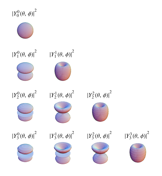
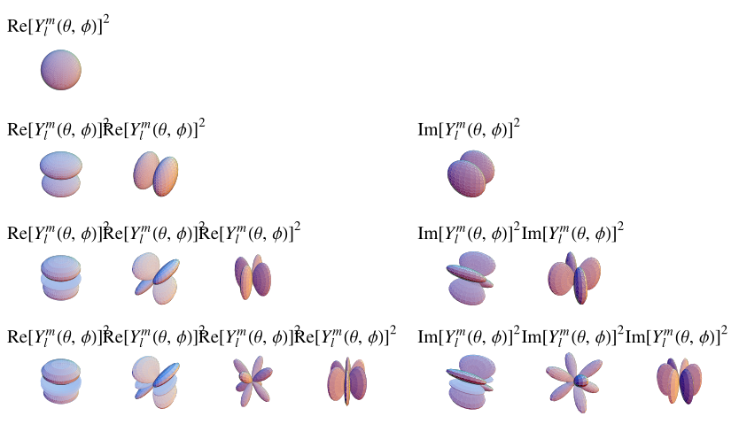
 (top),
 ![R[Y_l^m(theta,phi)]^2](/images/equations/SphericalHarmonic/Inline46.svg) (bottom left), and
(bottom left), and ![I[Y_l^m(theta,phi)]^2](/images/equations/SphericalHarmonic/Inline47.svg) (bottom right). The first few spherical
harmonics are
(bottom right). The first few spherical
harmonics are


 .
The sectorial harmonics are of
the form
.
The sectorial harmonics are of
the form

