Logistic Map

The logistic map is the quadratic recurrence equation obtained by replacing the logistic equation

with

where (sometimes also denoted ) is a real number. For positive , it is sometimes known as the "biotic potential". This quadratic map is capable of very complicated behavior. While John von Neumann had suggested using the logistic map as a random number generator in the late 1940s, it was not until work by W. Ricker in 1954 and detailed analytic studies of logistic maps beginning in the 1950s with Paul Stein and Stanislaw Ulam that the complicated properties of this type of map beyond simple oscillatory behavior were widely noted (Wolfram 2002, pp. 918-919).

The first few iterations of the logistic map (2) give

where is the initial value, plotted above through five iterations (with increasing iteration number indicated by colors; 1 is red, 2 is yellow, 3 is green, 4 is blue, and 5 is violet) for various values of .

The logistic map computed using a graphical procedure (Tabor 1989, p. 217) is known as a web diagram. A web diagram showing the first hundred or so iterations of this procedure and initial value appears on the cover of Packel (1996; left figure) and is animated in the right figure above.

Wolfram (2002, p. 1098) gives the formal representation

where satisfies and is a chosen branch of its inverse function. Elementary solutions for r=-2, r=2, and r=4 are summarized below (Wolfram 2002, p. 1098).

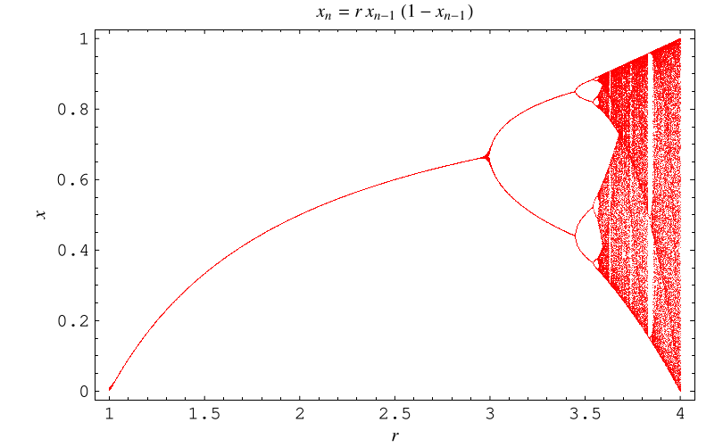
The illustration above shows a bifurcation diagram of the logistic map obtained by plotting as a function of a series of values for obtained by starting with a random number , iterating many times, and discarding the first points corresponding to values before the iterates converge to the attractor. In other words, the long-term iterates corresponding to a given value of are plotted for values of increasing to the right.

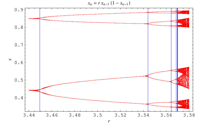
An enlargement of the previous diagram around is illustrated above, with value of at which a -cycle first appears indicated by blue lines.

To study the fixed points of the logistic map for positive , let an initial point lie in the interval . Now find appropriate conditions on which keep points in the interval. The maximum value can take is found from

so the largest value of occurs for . Plugging this in, . Therefore, to keep the map in the desired region, we must have . The magnitude of the Jacobian is

and a fixed point is locally asymptotically stable if .

Now find the fixed points of the map, which occur when . For convenience, drop the subscript on

so the fixed points are and .

At , the nonzero fixed point loses stability and the map undergoes a period doubling bifurcation with one stable orbit of period two for , corresponding to the two stable fixed points of . The fixed points of order two must satisfy , so

For convenience, drop the subscripts and rewrite

Notice that we have found the first-order fixed points as well, since two iterations of a first-order fixed point produce a trivial second-order fixed point. The true 2-cycles are given by solutions to the quadratic equation

These solutions are only real for , so this is where the 2-cycle begins. The 2-cycle can also be found from

The discriminant of the corresponding monic polynomial is

When this equals 0, two roots coincide, so is the onset of period doubling. For , the solutions are given by (0, 0, ) and (, , 3), so the first bifurcation occurs at .

In general, the set of equations which can be solved to give the onset of an -cycle by a fold bifurcation (Saha and Strogatz 1995) is

The first equations describe an orbit of period dividing . To obtain an -cycle, solutions of smaller period must be excluded. At the fold bifurcation, the derivative of at the orbit is 1. At a period doubling bifurcation, this derivative is . For small , these can be solved exactly, but the complexity rapidly increases with .

Now look for the onset of the 3-cycle. To eliminate the 1-cycles, consider

This gives

The roots of this equation are all nonreal for . At , two period-three orbits coincide and then separate into real orbits for larger . The value of can be found by computing the discriminant of the monic polynomial obtained from (26),

When the discriminant is zero, two roots coincide. This happens at

(OEIS A086178) as first shown by Myrberg in 1958, so the 3-cycle starts at . Saha and Strogatz (1995) give a simplified algebraic treatment for the 3-cycle which involves solving

together with three other simultaneous equations, where , , and . Further simplifications still are provided in Bechhoefer (1996) and Gordon (1996), but neither of these techniques generalizes easily to higher cycles. Bechhoefer (1996) expresses the three additional equations as

giving

This has the positive solution found previously, .

Gordon (1996) derives not only the value for the onset of the 3-cycle, but also an upper bound for the -values supporting stable period-3 orbits. This value is related to the unique positive root of the cubic equation

by

which is the unique positive root of the sextic polynomial

(OEIS A086179). For ,

Solving the resulting cubic equation using computer algebra gives

and , , given by

giving roots

Here, is the silver constant.

To find the onset of the 4-cycle, eliminate the 2- and 1-cycles by considering

This gives a 12th-order polynomial in . The value of can be found by computing the discriminant of the monic polynomial obtained from this polynomial,

whose only positive real roots are

The 4-cycle therefore starts at

(OEIS A086180).

The onset of 5-cycles can be found analytically, and gives a 22nd-order polynomial in whose positive real roots are (OEIS A118452), 3.90557..., and 3.99026....

The onset of 6-cycles can be found analytically, and gives a 40th-order polynomial in whose positive real roots are (OEIS A118453), 3.93751..., 3.97776..., and 3.99758....

The onset of 7-cycles can be found analytically, and gives a 114th-order polynomial in whose positive real roots are (OEIS A118746), 3.77413..., 3.88602..., 3.92218..., 3.95102..., 3.96897..., 3.98474..., 3.99453..., and 3.99939....

The onset of 8-cycles can be found analytically as the polynomial root of the 12th-order polynomial

(OEIS A086181; Bailey 1993; Bailey and Broadhurst 2000; Borwein and Bailey 2003, pp. 51-52).

The onset of 16-cycles at (OEIS A091517) was originally found using an integer relation calculation which determined that is the root of a 120th-degree integer polynomial with coefficients that decrease monotonically from to 1 (Bailey and Broadhurst 2000; Borwein and Bailey 2003, pp. 52-53). This result was subsequently verified exactly using computer algebra (Borwein and Bailey 2003, p. 53; Kotsireas and Karamanos 2004), and is an algebraic number of degree 240.

The following table summarizes the values at which the -cycle first appears. For , 2, ..., their minimal polynomials have degrees 1, 1, 2, 2, 22, 40, 114, 12, ... (OEIS A118454).

The degrees of the minimal polynomials of (i.e., the onset of the -cycle) for , 2, ... are therefore given by 1, 2, 12, 240, ... (OEIS A087046). A table of the cycle type and value of at which the -cycle appears is given below.

For additional values, see Rasband (1990, p. 23). Note that the table in Tabor (1989, p. 222) is incorrect, as is the entry in Lauwerier (1991). The period doubling bifurcations come faster and faster (8, 16, 32, ...), then suddenly break off. Beyond a certain point known as the accumulation point, periodicity gives way to chaos, as illustrated below. In the middle of the complexity, a window suddenly appears with a regular period like 3 or 7 as a result of mode locking. The period-3 bifurcation occurs at , and period doublings then begin again with cycles of 6, 12, ... and 7, 14, 28, ..., and then once again break off to chaos. However, note that considerable structure can be found within this chaos (Mayoral and Robledo 2005ab).

It is relatively easy to show that the logistic map is chaotic on an invariant Cantor set for (Devaney 1989, pp. 31-50; Gulick 1992, pp. 112-126; Holmgren 1996, pp. 69-85), but in fact, it is also chaotic for all (Robinson 1995, pp. 33-37; Kraft 1999).

At the accumulation point of the period doubling cascade, the attractor of the logistic map has reported correlation exponent (Grassberger and Procaccia 1983), capacity dimension 0.538 (Grassberger 1981), and information dimension 0.5170976 (Grassberger and Procaccia 1983).

The logistic map can be used to generate random numbers (Umeno 1998; Andrecut 1998; Gonzáles and Pino 1999, 2000; Gonzáles et al. 2001ab; Wong et al. 2001, Trott 2004, p. 105).