


Gaussian elimination is a method for solving matrix equations of the form
 |
(1)
|
More generally, Gaussian elimination applies to matrices over any field, including a finite field (Shoup 2009). For a dense
 matrix, the standard algorithm uses
  arithmetic operations, while pivoting
determines which element is used (Golub and Van Loan 2013). The row eliminations
associated with a given pivot can be performed in
parallel. De Laurentis and Franklin (2026) describe a parallel CUDA implementation
over finite fields, the real
numbers, and the complex numbers.
arithmetic operations, while pivoting
determines which element is used (Golub and Van Loan 2013). The row eliminations
associated with a given pivot can be performed in
parallel. De Laurentis and Franklin (2026) describe a parallel CUDA implementation
over finite fields, the real
numbers, and the complex numbers.
To perform Gaussian elimination starting with the system of equations
![[a_(11) a_(12) ... a_(1k); a_(21) a_(22) ... a_(2k); | | ... |; a_(k1) a_(k2) ... a_(kk)][x_1; x_2; |; x_k]=[b_1; b_2; |; b_k],](/images/equations/GaussianElimination/NumberedEquation2.svg) |
(2)
|
compose the "augmented matrix equation"
![[a_(11) a_(12) ... a_(1k); a_(21) a_(22) ... a_(2k); | | ... |; a_(k1) a_(k2) ... a_(kk)|b_1; b_2; |; b_k][x_1; x_2; |; x_k].](/images/equations/GaussianElimination/NumberedEquation3.svg) |
(3)
|
Here, the column vector in the variables  is carried along for labeling the matrix rows. Now, perform
elementary row operations to
put the augmented matrix into the upper
triangular form
is carried along for labeling the matrix rows. Now, perform
elementary row operations to
put the augmented matrix into the upper
triangular form
![[a_(11)^' a_(12)^' ... a_(1k)^'; 0 a_(22)^' ... a_(2k)^'; | | ... |; 0 0 ... a_(kk)^'|b_1^'; b_2^'; |; b_k^'].](/images/equations/GaussianElimination/NumberedEquation4.svg) |
(4)
|
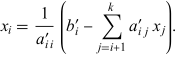
Solve the equation of the  th row for
  , then substitute back into the equation of the
  st row to obtain a solution for
  , etc., according to the formula
 |
(5)
|
In the Wolfram Language, RowReduce performs a version of Gaussian elimination, with the equation  being solved by
  GaussianElimination[m_?MatrixQ, v_?VectorQ] :=
    Last /@ RowReduce[Flatten /@ Transpose[{m, v}]]
LU decomposition of a matrix is frequently used as part of a Gaussian elimination process for solving a matrix equation.
A matrix that has undergone Gaussian elimination is said to be in echelon form. Continuing the process by normalizing each pivot and eliminating entries both above and below it produces reduced row-echelon form and is usually called Gauss-Jordan elimination.
For example, consider the matrix equation
![[9 3 4; 4 3 4; 1 1 1][x_1; x_2; x_3]=[7; 8; 3].](/images/equations/GaussianElimination/NumberedEquation6.svg) |
(6)
|
In augmented form, this becomes
![[9 3 4; 4 3 4; 1 1 1|7; 8; 3][x_1; x_2; x_3].](/images/equations/GaussianElimination/NumberedEquation7.svg) |
(7)
|
Switching the first and third rows (without switching the elements in the right-hand column vector) gives
![[1 1 1; 4 3 4; 9 3 4|3; 8; 7][x_1; x_2; x_3].](/images/equations/GaussianElimination/NumberedEquation8.svg) |
(8)
|
Subtracting 9 times the first row from the third row gives
![[1 1 1; 4 3 4; 0 -6 -5| 3; 8; -20][x_1; x_2; x_3].](/images/equations/GaussianElimination/NumberedEquation9.svg) |
(9)
|
Subtracting 4 times the first row from the second row gives
![[1 1 1; 0 -1 0; 0 -6 -5| 3; -4; -20][x_1; x_2; x_3].](/images/equations/GaussianElimination/NumberedEquation10.svg) |
(10)
|
Finally, adding  times the second row to the third row gives
![[1 1 1; 0 -1 0; 0 0 -5| 3; -4; 4][x_1; x_2; x_3].](/images/equations/GaussianElimination/NumberedEquation11.svg) |
(11)
|
Restoring the transformed matrix equation gives
![[1 1 1; 0 -1 0; 0 0 -5][x_1; x_2; x_3]=[ 3; -4; 4],](/images/equations/GaussianElimination/NumberedEquation12.svg) |
(12)
|
which can be solved immediately to give  , back-substituting to obtain
  (which actually follows trivially in this example), and
then again back-substituting to find
(which actually follows trivially in this example), and
then again back-substituting to find 
